Physics Solver

Analysis

This problem consists of three parts covering fundamental physics principles:

• Density and Geometry: Calculating the density of a solid cone using mass, height, and radius relationships.

• Vector Resolution: Finding the resultant of multiple vectors by resolving them into horizontal (x) and vertical (y) components.

• Kinematics: Analyzing the motion of a car using a speed-time graph and the principle that the area under the graph equals the total distance traveled.

---

Solution

Part (a)

1. Convert units to SI units (kg and m):

• Mass: $m = 2.5 \times 10^5 \text{ g} = \frac{2.5 \times 10^5}{1000} \text{ kg} = 250 \text{ kg}$

• Height: $h = 2.5 \times 10^3 \text{ mm} = \frac{2.5 \times 10^3}{1000} \text{ m} = 2.5 \text{ m}$

• Radius: $r = \frac{1}{3}h = \frac{1}{3}(2.5 \text{ m}) = 0.8333... \text{ m}$

2. Calculate the volume of the cone:
The formula for the volume of a cone is $V = \frac{1}{3} \pi r^2 h$.
$V = \frac{1}{3} \pi \left( \frac{2.5}{3} \right)^2 (2.5)$
$V = \frac{1}{3} \pi \left( \frac{6.25}{9} \right) (2.5)$
$V = \frac{15.625 \pi}{27} \approx 1.818 \text{ m}^3$

3. Calculate the density:
\rho = \frac{m}{V} = \frac{250}{1.818} \approx 137.51 \text{ \frac{kg}{m}}^3

---

Part (b)

1. Resolve each vector into components:

• Vector $\vec{A}$ (200 units, $28^\circ$ with +x):
  $A_x = 200 \cos(28^\circ) \approx 176.59$
  $A_y = 200 \sin(28^\circ) \approx 93.89$

• Vector $\vec{B}$ (150 units, $50^\circ$ with -x):
  $B_x = -150 \cos(50^\circ) \approx -96.42$
  $B_y = 150 \sin(50^\circ) \approx 114.91$

• Vector $\vec{C}$ (100 units, along -y):
  $C_x = 0$
  $C_y = -100$

• Vector $\vec{D}$ (50 units, $60^\circ$ with -y):
  $D_x = 50 \sin(60^\circ) \approx 43.30$
  $D_y = -50 \cos(60^\circ) = -25.00$

2. Sum the components:

• $R_x = \sum V_x = 176.59 - 96.42 + 0 + 43.30 = 123.47$

• $R_y = \sum V_y = 93.89 + 114.91 - 100 - 25.00 = 83.80$

3. Calculate Magnitude and Direction:

• Magnitude: $R = \sqrt{R_x^2 + R_y^2} = \sqrt{123.47^2 + 83.80^2} \approx 149.22 \text{ units}$

• Direction: $\theta = \arctan\left( \frac{R_y}{R_x} \right) = \arctan\left( \frac{83.80}{123.47} \right) \approx 34.16^\circ$ above the positive x-axis.

---

Part (c)

(i) Sketch the speed–time graph:

• Initial speed: 72 \text{ \frac{km}{h}} = \frac{72 \times 1000}{3600} \text{ \frac{m}{s}} = 20 \text{ \frac{m}{s}}.

• Total distance: $6 \text{ km} = 6000 \text{ m}$.

• Journey phases:

  • $t = 0$ to $45 \text{ s}$: Constant speed 20 \text{ \frac{m}{s}}.

  • $t = 45$ to $125 \text{ s}$ ($\Delta t = 80 \text{ s}$): Uniform acceleration to $v_{max}$.

  • $t = 125$ to $140 \text{ s}$ ($\Delta t = 15 \text{ s}$): Constant speed $v_{max}$.

  • $t = 140$ to $150 \text{ s}$ ($\Delta t = 10 \text{ s}$): Uniform deceleration to rest.

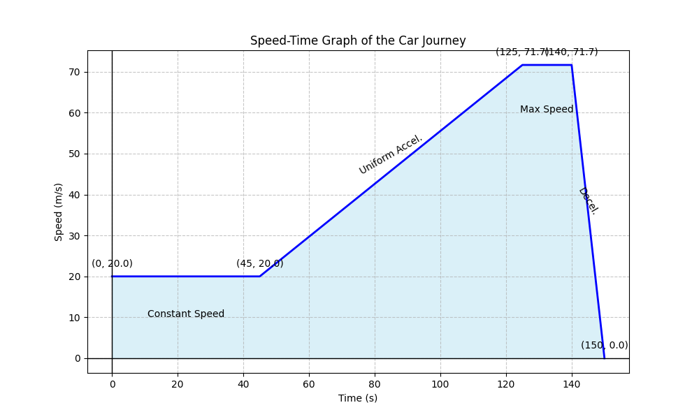
(ii) Determine the maximum speed:
The total distance is the area under the speed-time graph.

• Area 1 (Rectangle): $s_1 = 20 \times 45 = 900 \text{ m}$

• Area 2 (Trapezium): $s_2 = \frac{20 + v_{max}}{2} \times 80 = 40(20 + v_{max}) = 800 + 40v_{max}$

• Area 3 (Rectangle): $s_3 = 15 \times v_{max}$

• Area 4 (Triangle): $s_4 = \frac{1}{2} \times 10 \times v_{max} = 5v_{max}$

Summing the distances:
$900 + 800 + 40v_{max} + 15v_{max} + 5v_{max} = 6000$
$1700 + 60v_{max} = 6000$
$60v_{max} = 4300$
v_{max} = \frac{430}{6} \approx 71.67 \text{ \frac{m}{s}}

---

Answer

a) The density of the material is 137.51 \text{ \frac{kg}{m}}^3.

b) The resultant vector has a magnitude of $149.22 \text{ units}$ and a direction of $34.16^\circ$ relative to the positive x-axis.

c) (ii) The maximum speed of the car is 71.67 \text{ \frac{m}{s}}.

Analysis

This is a classical mechanics problem involving a block on an inclined plane. To find the maximum angle (often called the angle of repose) before the block begins to slide, we must analyze the forces acting on the block in a state of impending motion.

The primary physical principles involved are:

• Newton’s Second Law: Since we are looking for the limit of static equilibrium, the sum of forces in both the horizontal (parallel to the incline) and vertical (normal to the incline) directions must be zero.

• Friction Law: The maximum static friction force is proportional to the normal force, defined by the equation $f_s = \mu_s F_N$.

• Gravity Decomposition: Gravity acts vertically downward and must be resolved into components parallel and perpendicular to the inclined surface.

We will demonstrate that the mass of the block does not affect the maximum angle, as it cancels out during the algebraic derivation.

---

Solution

Step 1: Identify the forces acting on the block.
There are three main forces acting on the block:

• The force of gravity (weight), $W = mg$, acting straight down.

• The normal force, $F_N$, acting perpendicular to the surface of the incline.

• The static friction force, $f_s$, acting up the incline, opposing the tendency of the block to slide down.

Step 2: Resolve the weight into components.
We define a coordinate system where the $x$-axis is parallel to the incline and the $y$-axis is perpendicular to it. If $\theta$ is the angle of the incline:

• The component of weight perpendicular to the incline is $W_y = mg \cos \theta$.

• The component of weight parallel to the incline (pulling it down) is $W_x = mg \sin \theta$.

Step 3: Establish equilibrium equations.
For the block to remain stationary, the sum of forces in both directions must be zero.
Perpendicular to the incline ($y$-direction):
$\sum F_y = F_N - mg \cos \theta = 0$
$F_N = mg \cos \theta$

Parallel to the incline ($x$-direction) at the maximum angle:
$\sum F_x = mg \sin \theta - f_s = 0$
$f_s = mg \sin \theta$

Step 4: Apply the coefficient of friction.
The maximum static friction is reached just before the block slides, defined as:
$f_s = \mu_s F_N$
Substituting the expressions for $f_s$ and $F_N$ from Step 3:
$mg \sin \theta = \mu_s (mg \cos \theta)$

Step 5: Solve for the angle $\theta$.
Notice that the mass $m$ and gravity $g$ appear on both sides of the equation. We can divide both sides by $mg \cos \theta$:
$\frac{mg \sin \theta}{mg \cos \theta} = \mu_s$
$\tan \theta = \mu_s$
$\theta = \arctan(\mu_s)$

Step 6: Calculate the numerical value.
Given the coefficient of friction $\mu_s = 0.4$:
$\theta = \arctan(0.4)$
Using a calculator:
$\theta \approx 21.801^\circ$

---

Answer

The maximum angle of the incline before the block begins to slide is determined solely by the coefficient of friction and is independent of the block's mass.

$\theta = \arctan(0.4) \approx 21.8^\circ$

Šeit ir fizikas uzdevuma risinājums soli pa solim.

[Analysis]

Šis uzdevums prasa nolasīt mērierīču (voltmetra un ampērmetra) rādījumus, uzzīmēt atbilstošu elektrisko shēmu un aprēķināt rezistora pretestību, izmantojot Oma likumu.

• Mērierīču nolasīšana: Vispirms jānosaka katras mērierīces iedaļas vērtība (vismazākā iedaļa) un pēc tam jānolasa rādītāja pozīcija.

• Elektriskā shēma: Standarta ķēdē pretestības mērīšanai ietilpst strāvas avots, rezistors, ampērmetrs (pieslēgts virknē) un voltmetrs (pieslēgts paralēli rezistoram).

• Oma likums: Pretestību aprēķina pēc formulas $R = \frac{U}{I}$, kur $U$ ir spriegums un $I$ ir strāvas stiprums.

---

[Solution]

1. Voltmetra rādījuma (U) noteikšana

• Voltmetra skala ir no $0$ līdz $6 \text{ V}$.

• Starp lielajām iedaļām (piemēram, starp 4 un 5) ir redzamas $10$ mazas iedaļas.

• Vienas iedaļas vērtība voltmetram:
  $\text{Iedaļas vērtība}_V = \frac{5 \text{ V} - 4 \text{ V}}{10} = 0,1 \text{ V}$.

• Rādītājs atrodas uz 4. mazās iedaļas aiz skaitļa 4.

• Spriegums: $U = 4 \text{ V} + 4 \times 0,1 \text{ V} = 4,4 \text{ V}$.

2. Ampērmetra iedaļas vērtības un rādījuma (I) noteikšana

• Attēla augšdaļā redzamais ampērmetrs ir ar skalu no $0$ līdz $0,6 \text{ A}$.

• Starp skaitļiem $0,4$ un $0,5$ ir $10$ mazas iedaļas.

• Ampērmetra iedaļas vērtība:
  $\text{Iedaļas vērtība}_A = \frac{0,5 \text{ A} - 0,4 \text{ A}}{10} = 0,01 \text{ A}$.

• Rādītājs atrodas uz 4. mazās iedaļas aiz skaitļa 0,4.

• Strāvas stiprums: $I = 0,4 \text{ A} + 4 \times 0,01 \text{ A} = 0,44 \text{ A}$.

3. Rezistora pretestības (R) aprēķināšana

• Izmantojam Oma likumu ķēdes posmam: $R = \frac{U}{I}$.

• Ievietojam iegūtās vērtības:
  $R = \frac{4,4 \text{ V}}{0,44 \text{ A}} = 10 \text{ } \Omega$.

4. Elektriskās ķēdes shēma

• Shēmā tiek attēlots strāvas avots (baterija), rezistors, ampērmetrs virknē un voltmetrs paralēli rezistoram.

• Strāva plūst no pozitīvā (+) pola uz negatīvo (-) polu (atzīmēts ar bultiņu).

---

[Answer]

• Elektriskās ķēdes shēma: Shēma sastāv no strāvas avota, rezistora, ampērmetra (virknē) un voltmetra (paralēli rezistoram). Strāvas virziens ir no pozitīvā pola uz negatīvo.

• Ampērmetra iedaļas vērtība: $0,01 \text{ A}$.

• Rezistora pretestība: $R = 10 \text{ } \Omega$. Aprēķins: $R = \frac{4,4 \text{ V}}{0,44 \text{ A}} = 10 \text{ } \Omega$. Vērtības iegūtas, nosakot mērierīču iedaļas vērtību (voltmetram $0,1 \text{ V}$, ampērmetram $0,01 \text{ A}$) un nolasot rādītāju stāvokli.

Analysis

This problem involves understanding the difference between temperature and the perception of heat.

• Thermal Equilibrium: According to the problem statement, all objects are placed in a $500^\circ\text{F}$ ($260^\circ\text{C}$) oven and allowed to reach thermal equilibrium. This means that, initially, every object is at the exact same temperature of $260^\circ\text{C}$.

• Perception of "Hotness": When you touch an object, the "hotness" you feel is not a direct measurement of the object's temperature. Instead, your nerves respond to the rate of heat transfer into your skin and the resulting interface temperature at the point of contact.

• Thermal Conductivity ($k$): The primary factor determining how fast heat moves from the bulk of the object into your hand is its thermal conductivity. Materials with high thermal conductivity (like metals) can replenish heat at the contact surface very quickly, keeping the interface temperature high and transferring more energy per second. Materials with low thermal conductivity (insulators like wood or steak) cannot move heat to the surface quickly; thus, the surface in contact with your hand cools down rapidly, making the object feel "less hot."

• Thermal Effusivity: More technically, the interface temperature $T_i$ is determined by the thermal effusivity $\epsilon = \sqrt{k \rho c}$. However, because the thermal conductivity $k$ varies by several orders of magnitude between metals and insulators in this problem, it is the dominant factor for ranking.

Solution

Step 1: Identify the initial temperature of all objects.
Since all objects have reached thermal equilibrium with the oven at $260^\circ\text{C}$, their temperatures are all equal:
$T_{\text{glass}} = T_{\text{aluminum}} = T_{\text{wood}} = T_{\text{silver}} = T_{\text{steak}} = T_{\text{iron}} = 260^\circ\text{C}$

Step 2: Compare the thermal conductivity ($k$) values provided.
The sensation of heat is proportional to the rate of conduction. We list the values given in the image:

• Silver ingot: $k = 420 \text{ J/(s}\cdot\text{m}\cdot^\circ\text{C)}$

• Aluminum pot: $k = 220 \text{ J/(s}\cdot\text{m}\cdot^\circ\text{C)}$

• Iron skillet: $k = 80 \text{ J/(s}\cdot\text{m}\cdot^\circ\text{C)}$

• Glass casserole dish: $k = 0.8 \text{ J/(s}\cdot\text{m}\cdot^\circ\text{C)}$

• Well done steak: $k = 0.2 \text{ J/(s}\cdot\text{m}\cdot^\circ\text{C)}$

• Wooden cutting board: $k = 0.1 \text{ J/(s}\cdot\text{m}\cdot^\circ\text{C)}$

Step 3: Rank the objects based on the rate of heat transfer.
The object with the highest thermal conductivity will transfer heat to the hand the fastest and feel the hottest. The object with the lowest will feel the least hot.
Comparing the values:
$420 > 220 > 80 > 0.8 > 0.2 > 0.1$

Step 4: Formulate the final ranking.
The order from hottest feeling to least hot feeling is:

• Silver ingot (hottest)

• Aluminum pot

• Iron skillet

• Glass casserole dish

• Well done steak

• Wooden cutting board (least hot)

Answer

The ranking of the objects from how hot they feel (largest sensation of heat to smallest) is:
Silver ingot > Aluminum pot > Iron skillet > Glass casserole dish > Well done steak > Wooden cutting board